ENVSOCTY 4GA3 – Spatially Continuous Data II

Spatial dependence in spatially continuous data

Spatial interpolation assumes that the data exhibit positive spatial autocorrelation.
Single-scale autocorrelation measures, such as the global Moran’s I statistic, are not well-suited for spatially continuous data due to its smooth nature, where neighborhoods are not well-defined.
Consequently, a measure that quantifies autocorrelation at different scales is required.

Variographic analyisis

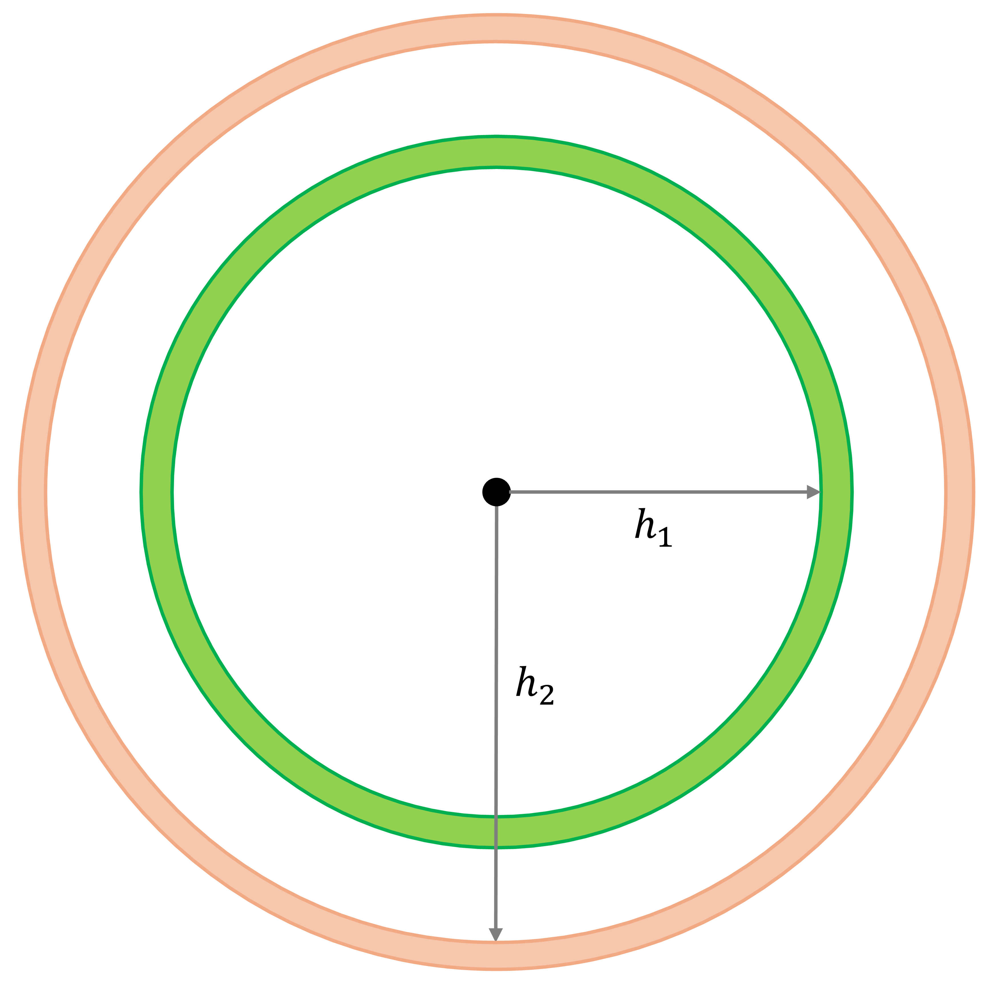
We define a binary spatial weight matrix as:

$w_{ij}(h)=\bigg\{\begin{array}{l l} 1\text{, if } d_{ij} = h\\ 0\text{, otherwise}\\ \end{array}$

Variographic analyisis

Autocovariance:

$C_{z}(h) = \frac{\sum_{i=1}^{n}{w_{ij}(h)(z_i^2 - \bar{z})(z_j^2 - \bar{z})}}{\sum_{i=1}^n{w_{ij}(h)}}$

Semivariance:

$\hat{\gamma}_{z}(h) = \frac{\sum_{i=1}^{n}{w_{ij}(h)(z_i - z_j)^2}}{2\sum_{i=1}^n{w_{ij}(h)}}$

Covariogram and semivariogram

Covariogram:

Semivariogram:

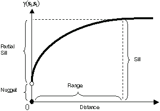
The autocovariance, $C_{z}(h)$ , and semivariance, $\hat{\gamma}_{z}(h)$ , are related as follows: $C_{z}(h) = \sigma^2 - \hat{\gamma}_{z}(h)$ where $\sigma^2$ is the sample variance.

Kriging

The theoretical spatial continuous process can be expressed as: $z_i = f(u_i, v_i) + \epsilon_i$

To interpolate, we use: $\hat{z_i} = \underbrace{\hat{f}(x_p, y_p)}_{\text{a smooth estimator, e.g., trend surface}} + \hat{\epsilon_p}$

Here, $\hat{\epsilon}_p = \sum_{i=1}^n {\lambda_{pi}\epsilon_i}$ and $\epsilon_i = z_i - \hat{f}(x_i, y_i)$ .

The expected mean squared error or prediction variance is: $\sigma_{\epsilon}^2 = E[(\hat{\epsilon}_p - \epsilon_i)^2]$ .

The expectation of the prediction errors is zero (unbiassedness) Find the weights $\lambda$ that minimize the prediction variance (optimal estimator).

Activities for today

We will work on the following chapter from the textbook:
- Chapter 36: Activity 17: Spatially Continuous Data III
- Chapter 38: Activity 18: Spatially Continuous Data IV
The hard deadline is Friday, March 28.

Reference

https://pro.arcgis.com/en/pro-app/latest/help/analysis/geostatistical-analyst/understanding-a-semivariogram-the-range-sill-and-nugget.htm