Policy and agenda
- You need to finish the weekly reading before coming to the lab.
- Activity is marked as satisfactory completion or not:
- Poor quality submissions will result in a 0.
- Suspicious AI-generated content will be flagged (manually) and forwarded to the professor.
- We will work on activities during the lab:
- The focus is more on how to code rather than on theories.
Packages we use today
Load the following three packages.
library(isdas)
library(sf)
library(tidyverse)
If you have trouble restoring the reproducible environment, you need to manually install the packages first.
install.packages("remotes")
remotes::install_github("paezha/isdas")

install.packages("sf")

install.packages("tidyverse")
What does each package do?
isdas: The course companion package containing all the data we will use.sf: The GIS package that enables us to work with vector data.tidyverse: A meta-package that encompasses plotting, data manipulation, and additional functionality.
ggplot2 package
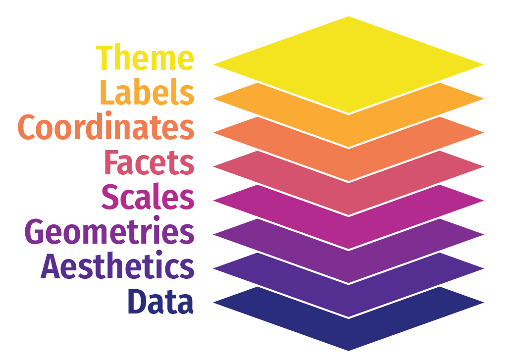
ggplot2 is one of the packages included in tidyverse.- It enables us to use the Grammar of Graphics to create plots.
- It creates plots through overlaying layers created using
geom_*.
How layering works?
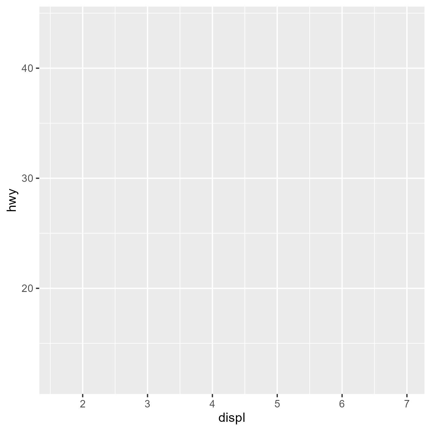
First, we create a canvas.
How layering works?
ggplot(data = mpg) +
  aes(x = displ,
      y = hwy)
Then, we assign which variables go to which axis.
How layering works?
ggplot(data = mpg) +
  aes(x = displ,
      y = hwy) +
  geom_point()
We add data points to the plot.
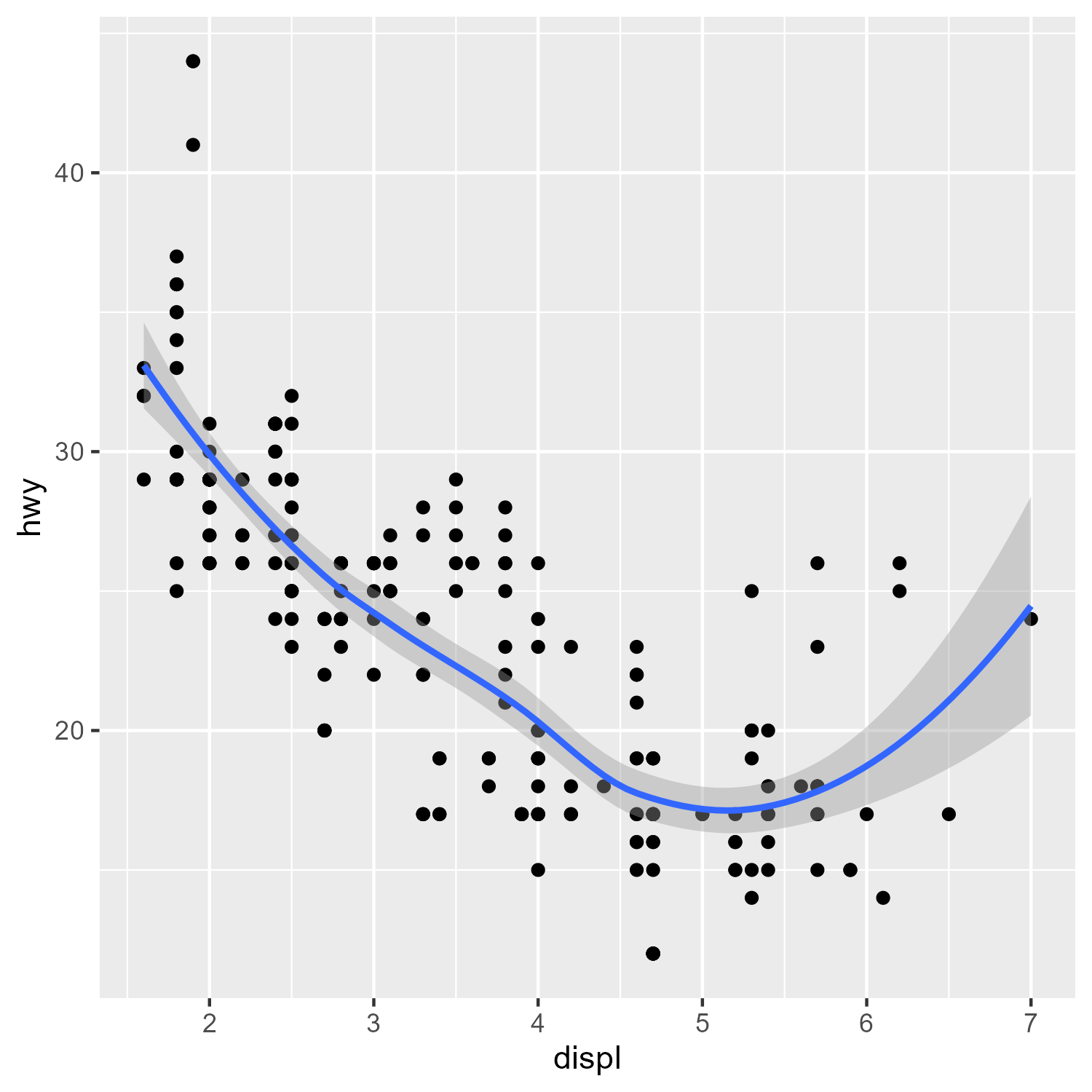
How layering works?
ggplot(data = mpg) +
  aes(x = displ,
      y = hwy) +
  geom_point() +
  geom_smooth()
Finally, we add an (default: local polynomial) regression line to the points.
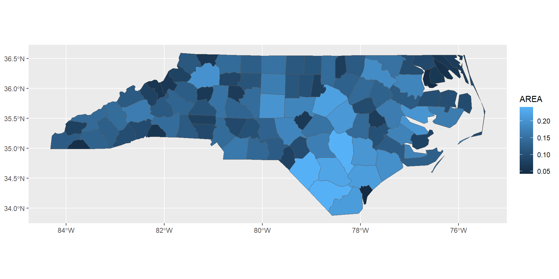
Mapping
Mapping an sf object (vector data) is straightforward. We use geom_sf for this purpose.
ggplot(data = nc) +
  geom_sf(aes(fill = AREA))
![]()
Activities for today
- We will work on the following chapter from the textbook:
- Chapter 4: Activity: Statistical Maps I
- Chapter 6: Activity 2: Statistical Maps II
- The hard deadline is Friday, January 24 (12:00 pm).