Time-Series OLS Estimation Bias

This project involved simulating the bias in ordinary least squares (OLS) estimation on time series data when it follows an autoregressive process of order one (AR(1)).

# load packages used in this post
library(tidyverse)
library(Hmisc)
library(latex2exp)

Time-series regression is a common method to analyze the relationship between a dependent variable and one or more independent variables over time. However, this method can be biased if the dependent variable follows an autoregressive process, which means that its current value depends on its past values. In this blog post, I will explore the nature and magnitude of this bias, following the work of Alex and Kendall (1954).

The first step is to generate data from an AR(1) process. An AR(1) process is defined by the following equation:

\[ \begin{array}{rl} y_t=&\rho y_{t-1}+u_t\\ where\ &u_t\sim N(0,1)\\ &y_0\sim N(0,1) \end{array} \] Due to the endogeneity issues, the OLS estimate for the following regression would produce biased estimate for \(\hat{\rho}\).

\[ y_t=\hat{\beta}_0+\hat{\rho}y_{t-1}+\epsilon_t \]

To generate data from this process and carry out estimation, I use the following R code:

ar1_bias <- function(n, rho, times) {
  return_df <- as.data.frame(matrix(nrow = times, ncol = length(rho)))
  colnames(return_df) <- gsub("-", "_", paste0("rho", rho))
  
  for (count in 1:times) {
    # create a dataframe to hold samples
    df <- as.data.frame(matrix(nrow = n, ncol = length(rho)))
    colnames(df) <- gsub("-", "_", paste0("rho", rho))
    
    for (i in 1:length(rho)) {
      df[1, i] <- rnorm(1)
      for(j in 2:n) {
        df[j, i] <- rho[i]*df[j-1, i] + rnorm(1)
      }
    }
    
    for (i in colnames(df)) {
      df[, paste0(i, "_1")] <- Lag(df[,i])
    }
    
    ols_estimate <- data.frame(rho = rho, rho_hat = NA)
    j <- 1
    
    for (i in gsub("-", "_", paste0("rho", rho))) {
      str_exp <- paste0(i, "~", i, "_1")
      exp_for <- as.formula(str_exp)
      holder <- lm(exp_for, data = df)
      ols_estimate[j,2] <- holder$coefficients[[2]]
      j <- j + 1
    }
    
    ols_estimate$diff <- ols_estimate$rho_hat - ols_estimate$rho
    return_df[count,] <- ols_estimate$diff
  }
  
  return(return_df)
}

The bias in the OLS estimation is calculated as

\[ \hat{Bias}=E(\hat{\rho}-\rho)=E(\hat{\rho})-\rho \]

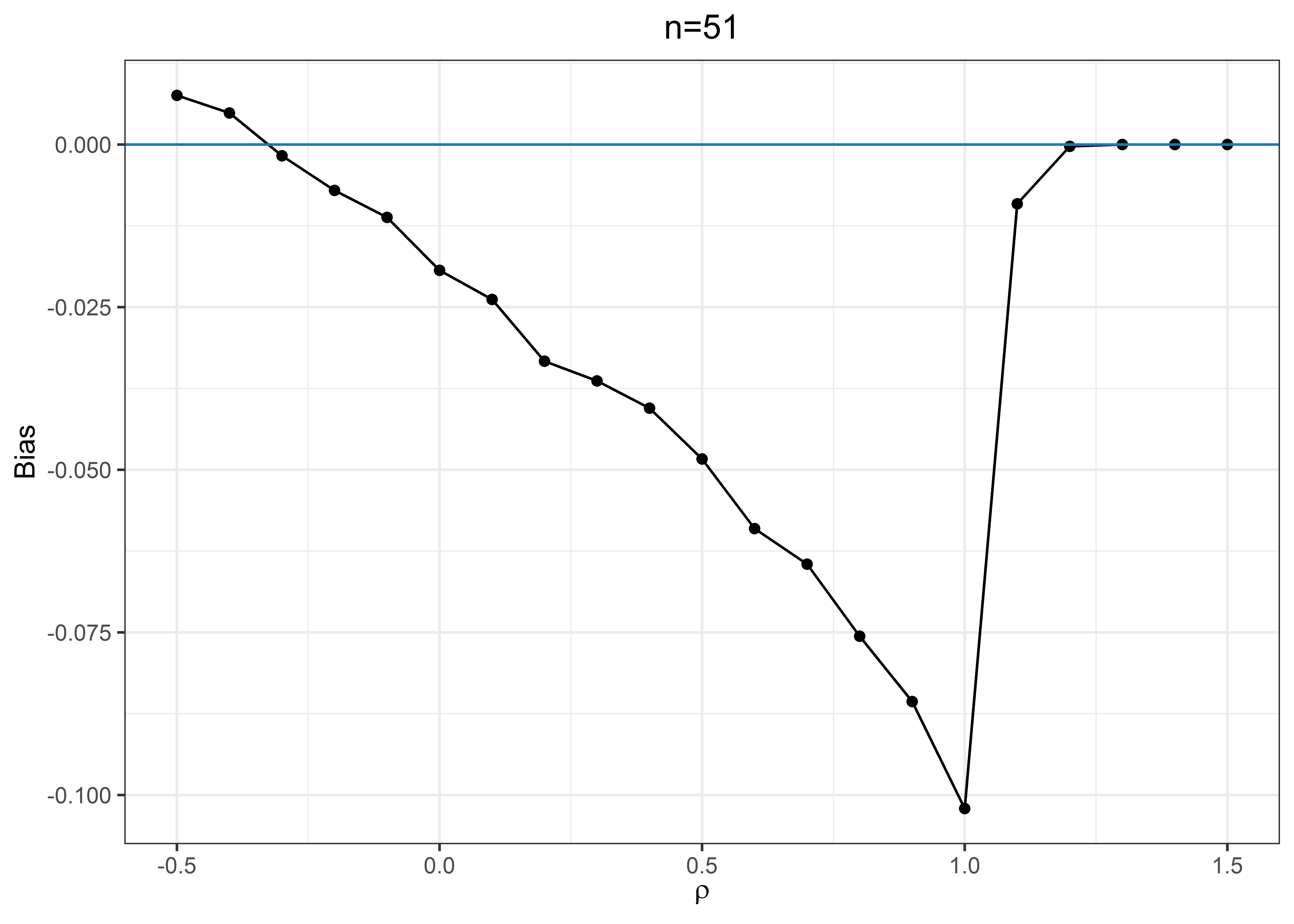
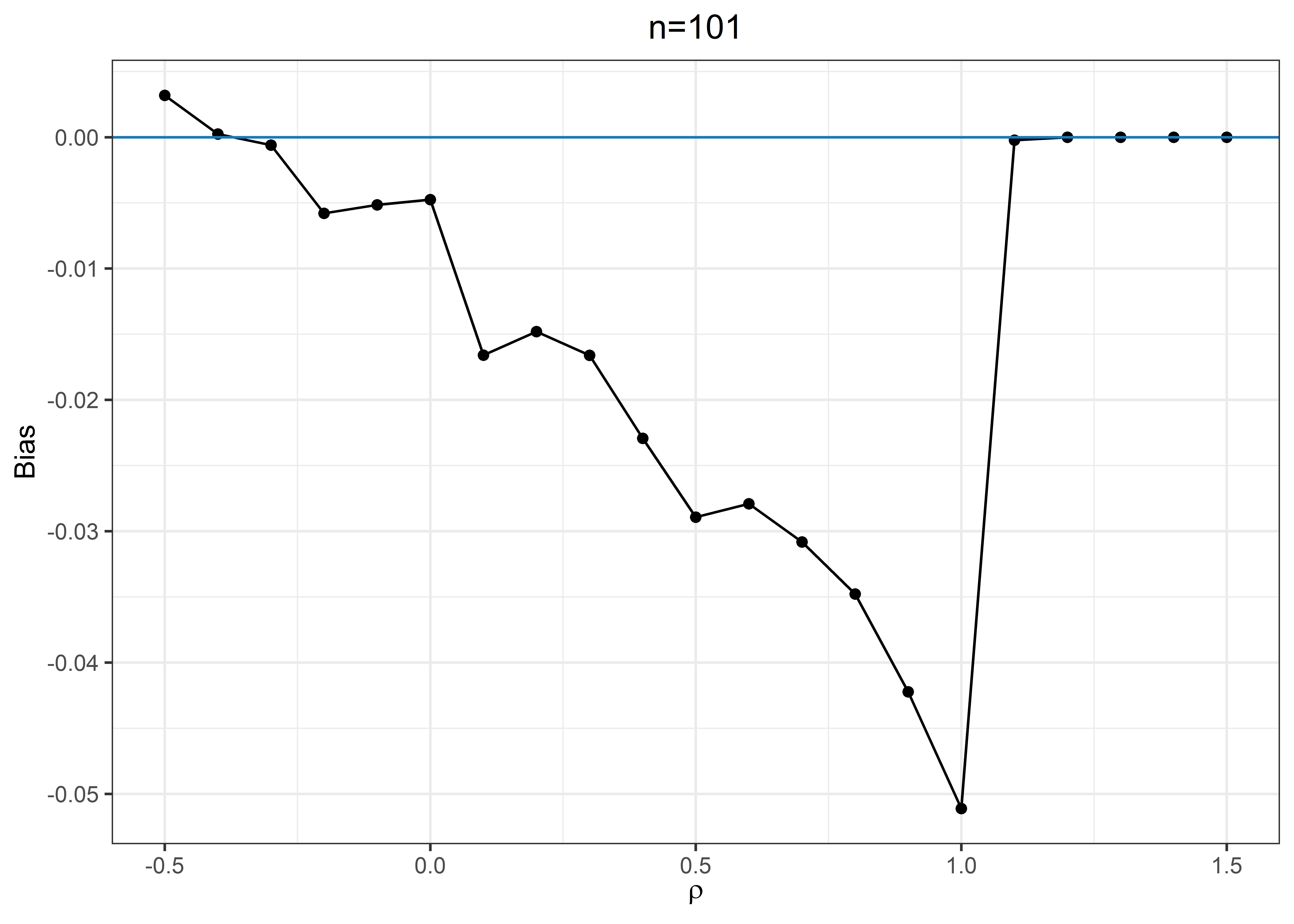
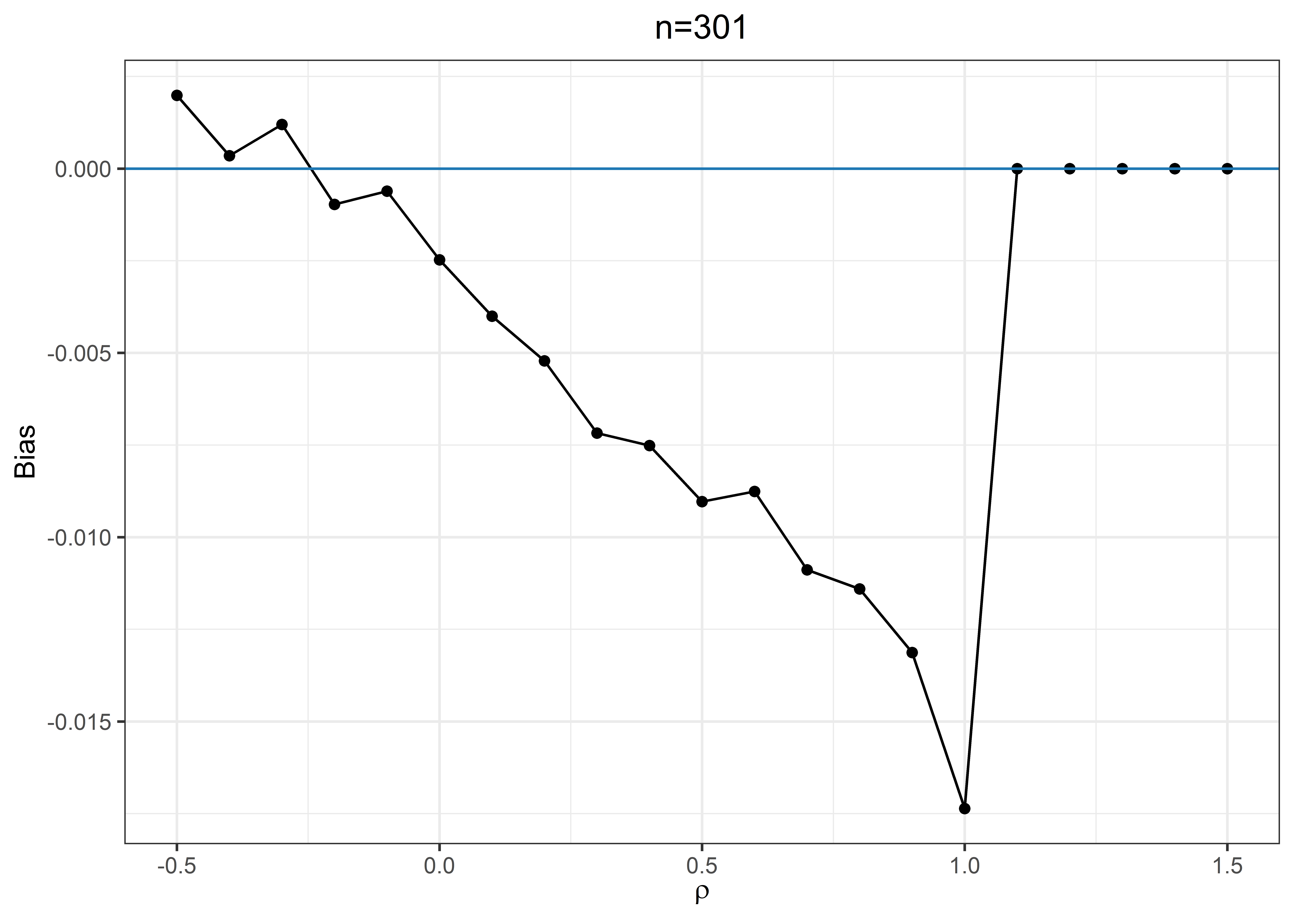
Here we carry out simulations for different values of \(\rho\) and sample size \(n\).

# for reproductivity
set.seed(123)

sim <- ar1_bias(n = 51, 
                rho = seq(-0.5, 1.5, 0.1), 
                times = 3000)

sim |>
  pivot_longer(everything(), names_to = "rho", values_to = "diff") |>
  mutate(rho = gsub("_", "-", rho)) |>
  mutate(rho = parse_number(rho)) |>
  group_by(rho) |>
  summarise(mean = mean(diff)) |>
  ggplot(aes(x = rho, y = mean)) + 
  geom_point() + geom_line() +
  geom_hline(yintercept = 0, color = "#1f78b4") +
  labs(x = TeX("$\\rho$"), y = "Bias",
       title = "n=51") +
  theme_bw() +
  theme(plot.title = element_text(hjust = 0.5))

sim <- ar1_bias(n = 101, 
                rho = seq(-0.5, 1.5, 0.1), 
                times = 3000)

sim |>
  pivot_longer(everything(), names_to = "rho", values_to = "diff") |>
  mutate(rho = gsub("_", "-", rho)) |>
  mutate(rho = parse_number(rho)) |>
  group_by(rho) |>
  summarise(mean = mean(diff)) |>
  ggplot(aes(x = rho, y = mean)) + 
  geom_point() + geom_line() +
  geom_hline(yintercept = 0, color = "#1f78b4") +
  labs(x = TeX("$\\rho$"), y = "Bias",
       title = "n=101") +
  theme_bw() +
  theme(plot.title = element_text(hjust = 0.5))

sim <- ar1_bias(n = 301, 
                rho = seq(-0.5, 1.5, 0.1), 
                times = 3000)

sim |>
  pivot_longer(everything(), names_to = "rho", values_to = "diff") |>
  mutate(rho = gsub("_", "-", rho)) |>
  mutate(rho = parse_number(rho)) |>
  group_by(rho) |>
  summarise(mean = mean(diff)) |>
  ggplot(aes(x = rho, y = mean)) + 
  geom_point() + geom_line() +
  geom_hline(yintercept = 0, color = "#1f78b4") +
  labs(x = TeX("$\\rho$"), y = "Bias",
       title = "n=301") +
  theme_bw() +
  theme(plot.title = element_text(hjust = 0.5))

Therefore, we can see the bias increases as the population parameter \(\rho\) approaches 1 and the bias persists even when \(\rho=0\). This casts some concerns for the time series data analysis.